Pi computation algorithms (2)

Date: 2025-08-14

Tags: C soft benchmark pi

We’ve seen multiple algorithms to compute approximations of $\pi$ in a previous article¹. Once we know they all work, we can compare them, making sure to run them on the same machine within the same conditions.

Getting data

Convergence

One important thing is to see how long an algorithm takes to converge, and make sure they converge. This needs to take the duration of each iteration of loops, as well as the number of iterations.

First, we can simply run our code, sweeping for different iteration numbers, and types of algorithms²:

for algo in circle taylor leibniz sphere euler agm newton_gmp \
machin_gmp archimedes_gmp ramanujan chudnovsky plouffe bellard;
    do for n in 1 2 3 10 30 100 300 1000;
        do ./pi $algo $n;
    done;
done > benchmark

We also need to make the file less human-readable and more machine-readable, to something similar to CSV³:

sed -i 's/\,\titerations\:\ /\t/g' benchmark
sed -i 's/,\tpi\ \=\ /\t/g' benchmark
sed -i 's/,\terr\ = /\t/g' benchmark

Execution times

We can compare execution times:

hyperfine --export-json benchmark.json -N -r 10 -w 1 -L algo circle,\
taylor,leibniz,sphere,euler,agm,newton,newton_gmp,machin,machin_gmp,\
archimedes,archimedes_gmp,ramanujan,chudnovsky,plouffe,bellard \
-L n 1,2,3,10,30,100,300,1000 "./pi {algo} {n}" -i

Hyperfine returns a JSON file that’s completely different than the CSV file we built. Having both execution times and accuracy in a single file would be nicer.

We can do that using jq wrapped around some bash code:

rm benchmark2.json;
for algo in circle taylor leibniz sphere euler agm newton_gmp \
machin_gmp archimedes_gmp ramanujan chudnovsky plouffe bellard;
    do for n in 1 2 3 10 30 100 300 1000;
        do pi=$(grep ^$algo$'\t'${n}$'\t' benchmark | awk '{ print $3}');
        diff=$(grep ^$algo$'\t'${n}$'\t' benchmark | awk '{ print $4}');
        echo $(cat benchmark.json |jq -r ".results[] | \
        select(.parameters.n == \"$n\" and .parameters.algo == \"$algo\") | \
        .pi="$pi" |.diff="$diff"")$',' >> benchmark2.json;
        # match parameters.n and parameters.algo from the json file with $n
        # and $algo from the csv file, adds $pi and $diff from the CSV file,
        # adds a comma and write to benchmark2.json
    done;
done;
sed -i '1s/^/{"results": [\n/' benchmark2.json; # adds a file header
sed -i '/^,$/d' benchmark2.json;    # remove commas from blank lines
truncate -s -2 benchmark2.json      # removes the last comma and \n
echo "\n]}" >> benchmark2.json      # closes brackets at the end of the file

This builds a new JSON file based on the content of the old JSON and CSV files.

Plots

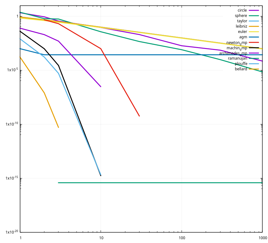
We can simply display the content of the CSV file with a line plot:

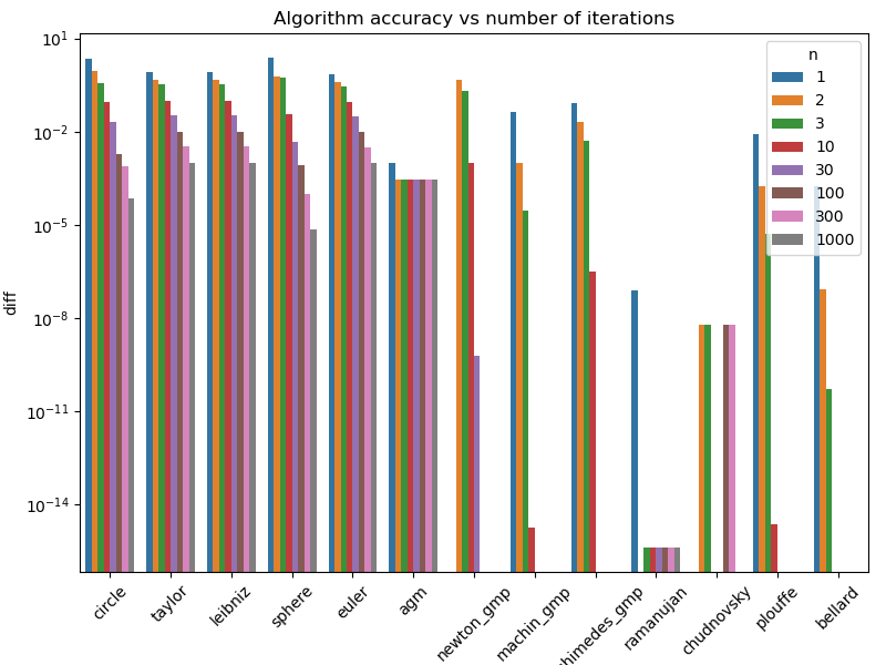
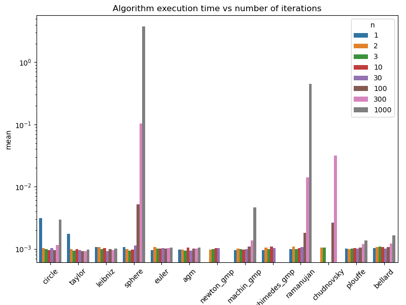
This shows everything, although it’s not easy to read. Instead, we can build a Python script to display the data we collected into the JSON file.

This gives barplots showing the execution time and the accuracy relative to the iteration number for each algorithm.

Both informations are interesting, but what’s important is actually the compromise between execution time and accuracy.

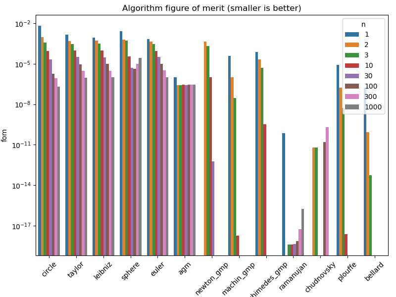
To address that, we can compute a figure of merit by multiplying the execution time and the accuracy, without any coefficients. In this case, a smaller number means that an algorithm is both quick and accurate.

First conclusions

That enables us rate algorithms, or actually their implementation, based a few things:

• Missing data:
  • Failed computation
  • Accuracy better than 64-bit numbers
• Convergence that stops: accuracy limited by implementation
• Convergence speed
• Increasing figure of merit after a number of iteration:
  • Stalled algorithm
  • Accuracy limited by implementation

Algorithm ratings

Algorithm	Accuracy	Figure of merit	Stops converging	Accuracy limited by 64-bit floats
Circle	Poor	Poor	-	-
Sphere	Average	Poor	-	-
Taylor	Poor	Poor	-	-
Machin	Good	Good	-	-
Leibniz	Poor	Poor	-	-
Euler	Poor	Poor	-	-
Gauss-AGM	Average	Average	Y	-
Newton	Good	Good	-	-
Archimedes	Average	Average	-	-
Ramanujan	Very Good	Very Good	Y	Y
Chudnovsky	Good	Average	Y
Plouffe	Very Good	Very Good	Y	Y
Bellard	Very Good	Very Good	Y	Y

Algorithms shown in bold can be implemented again for better results.

Algorithms shown in italic have been tested with gmp_printf() to get rid of the 64-bit float limit.

---

1. Pi computation algorithms - Monorailc.at↩︎

2. Long Bash command lines have been trimmed to roughly fit 80 columns to improve readability. Backslashes at the end of line aren’t mandatory.↩︎

3. It’s not proper CSV since we’re using tabs instead of commas↩︎

• ← Previous page
  Débimètre Bosch HFM
• Next page →
  cms

Electronics Électronique puissance semiconducteur semiconductors power Hardware CPE INSA Xavier Bourgeois

Xavier