Pi computation algorithms

Date: 2025-07-31

Tags: C soft benchmark

Last time I wrote a series of articles about comparing different programming languages, by using an algorithm to compute an approximated value of $\pi$.

This time, I’m going to use the same programming language to compare different algorithms, just to see if some need less iterations to converge, or can have faster iterations.

Since I’m going to copy-paste some algorithms, and write some exclusively from scratch, comparing the time it takes isn’t fair, so we’re going to compare the number of lines and the execution times instead.

Algorithms

Montecarlo

This algorithm has been described in a previous article¹, using both C and Python languages.

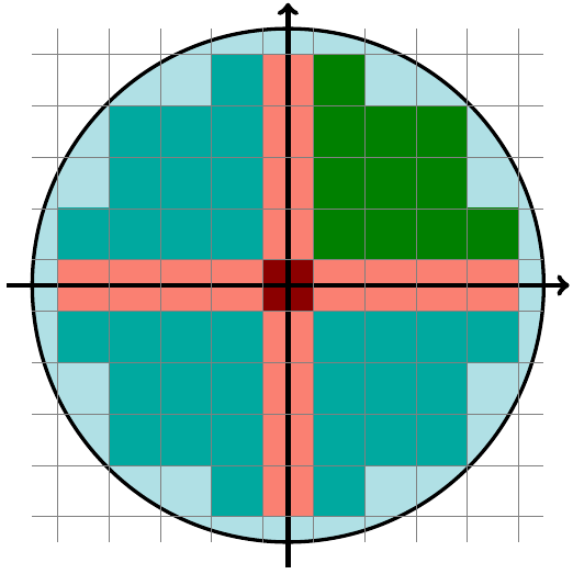
Circle

This algorithm has also been described in a previous article², using most languages I’ve heard of.

The idea is to compute $\pi$ using the ratio of the area of a disc, and its radius squared. The bigger the radius, the more accurate the approximation should be $S = r^2 $, which gives us:

$$\pi = \frac{S}{r^2}$$

This is straightforward to translate to C:

unsigned long count = 0;
int i, j;

for(i = -n; i <= n; i++) {
    for(j = -n; j <= n; j++) {
        if(i*i + j*j < n*n) {
            count++;
        }
    }
}
return (double) count / (n*n);

Sphere

Since we can compute $\pi$ using a disc, why not compute the volume of a sphere. It’s exactly the same idea with one more dimension.

$$\pi = \frac{3}{4} \frac{V}{r^3}$$

N-Sphere

Now that we started, why stop here? We can also compute the volume of a N-sphere, actually a N-Ball³⁴, and find $\pi$ with a relation between its volume and its radius.

Finding the relation between the volume and the radius may not be that straightforward, so we can split it for odd and even dimensions:

$$V_n = \begin{cases} \frac{1}{(\frac{n}{2})!} \cdot \pi^{\frac{n}{2}} \cdot R^n &\text{if } n &\text{is even}\\ \frac{2^{\frac{n+1}{2}}}{n!!} \cdot \pi^{\frac{n-1}{2}} \cdot R^n &\text{if } n &\text{is odd} \end{cases}$$

The algorithm contains sections of code that need to be broken down into 3 functions:

• nsphere(), gets all the parameters, counts the number of p-dimensions elements in a p-sphere split into n along each dimension, and computes $\pi$ based on that count and coefficients shown above
• compute_nd_sphere(), recursive function that counts elements by looping along one dimension, and calls itself for each lower dimension
• compute_1d_sphere(), non-recursive function that only loops once and is needed for all dimensions greater than one

Here’s how the main compute function looks like. It calls itself for each dimension, until it reaches the dimension 2, where it calls compute_1d_sphere().

unsigned long compute_nd_sphere(int n, int carry, unsigned short dim) {
    unsigned long count = 0;
    int i;

    if(dim < 2)
        return 0;
    if(dim == 2) {
        for(i = -n; i <= n; i++)
            count += compute_1d_sphere(-n, n, i*i + carry);
    }
    if(dim > 2) {
        for(i = -n; i <= n; i++)
            count += compute_nd_sphere(n, i*i + carry, dim-1, opt);
    }
    return count;
}

compute_1d_sphere() is exactly the same, except that it only sweeps along one dimension.

unsigned long compute_1d_sphere(int start, int stop, int carry) {
    unsigned long count = 0;
    int i;
    for(i = start; i <= stop; i++) {
        if(i*i + carry < stop*stop)
            count++;
    }
    return count;
}

Optimized N-Sphere

As we showed at the end of a previous article⁵, discs are symmetric around their center, and also along whichever axis that cuts their center.

For convenience, we can cut a disk in 4 quadrants, compute the area of one quadrant and multiply it by 4 to get the same result, using 4 times less computations.

A 3D-sphere can also be split in 8 quadrants, and going further, a N-sphere can be split in $2^N$ quadrants.

unsigned long compute_nd_sphere(int n, int carry, unsigned short dim, unsigned short opt) {
    unsigned long count = 0;
    int i;
    int start;
    if(opt == 1) {
        start = 1;

        if(dim < 2)
            return 0;
        if(dim == 2) {
            for(i = start; i <= n; i++)
                count += 4*compute_1d_sphere(1, n, i*i + carry);
        }
        if(dim > 2) {
            for(i = start; i <= n; i++)
                count += 2*compute_nd_sphere(n, i*i + carry, dim-1, opt);
        }
    }
    return count;
}

The major difference compared to the previous function, is the variable start that loops from 1 instead of -n, meaning it halves the number of computations for each dimension.

There’s one catch though. Counting discrete elements inside a shape can get tricky. We need to make sure no element is forgotten or counted twice.

On a disc, sweeping $4 \cdot n^2$ elements is straightforward, however simplifying and swiping from 0 to n on each axis means that each quadrant now overlaps, and swiping from 1 to n on each axis means that there’s a gap between each quadrant. The solution is intuitive : just add a missing cross that goes from -n to n on 2 axis, meaning $4n-1$, since we shouldn’t count the center twice.

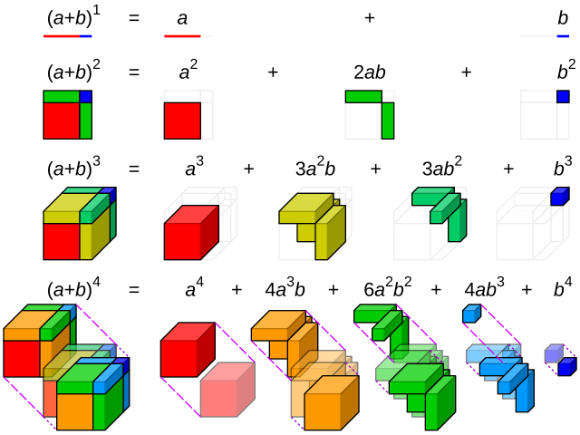
Things start getting complex when adding dimensions. With a 3D-sphere, we need to add slices that have the shape of a disc.

A brain-twister that took some time to understand was to see that in the same way as the area of a N-dimension rectangle⁶.

After some time, I found a generic formula that works with N-dimensions, and a radius r:

$$V_{lost}(N) = N \cdot V(N-1) + \sum_{i=2}^{N-2} \binom{N}{i} \cdot V(i) + 2 \cdot N \cdot r - 2 \cdot N + 1$$

Taylor

One way of computing $\pi$ is to use trigonometric functions, especially $arctan(1) = \frac{\pi}{4}$. And since $arctan(x)$ isn’t easy to use, we’ll approximate it using series of polynoms coming from the Taylor/McLaurin method⁷.

$$arctan(x) = \sum_{n=0} ^{\infty} \frac{(-1)^n}{2 n + 1} x^{2n+1}$$

That makes it easy for $x = 1$, where $arctan(1) = \frac{\pi}{4}$, where we can simplify it and write it in C.

unsigned long i;
int a = 1;
int b = 1;
double pi_4 = 0;
for(i = 0; i < n; i++) {
    pi_4 += (double) a / (double) b;
    a = -a;
    b += 2;
}
return pi_4 * 4.0;

a is the numerator, which alternates between $+1$ and $-1$, and b is the denominator, where we can translate $2n+1$ by starting with $1$ and adding $2$ for each iteration.

Each iteration has one division, two sums and one sign change. This takes very little computing power and is very fast. Though, it takes lots of iterations to converge.

Machin

Machin’s formula can be used with Taylor’s series⁸:

$$\frac{\pi}{4} = arctan(1) = 4 \cdot arctan(\frac{1}{5}) - arctan(\frac{1}{239})$$

Merging that with the Taylor series yields to:

$$\frac{\pi}{4} \sim 4\cdot \sum_{k=0} ^{n} \frac{(-1)^k}{(2 k + 1) \cdot 5^{2k+1}} - \sum_{k=0} ^{n} \frac{(-1)^k}{(2 k + 1) \cdot 239^{2k+1}}$$

This can be translated to C:

double machin(unsigned long n) {
    // Machin formula based on Taylor series 4*arctan(1/5) - arctan(1/239) = pi/4
    // unsigned long int is the limit
    unsigned long i;
    int a = -1;
    unsigned long int b = 0;
    unsigned long int c = 0;
    double pi_4 = 0;
    for(i = 0; i < n; i++) {
        a = -a;
        b = pow(5, 2*i+1) * (2*i+1);
        c = pow(239, 2*i+1) * (2*i+1);
        pi_4 += 4.0 * (double) a / (double) b - (double) a / (double) c;
    }
    return pi_4 * 4.0;

Except there’s a catch: $239^{2i+1}$ increases fast, and means that c will quickly overflow, actually for $n \geq 5$.

Improved resolution

Let’s try a way to use larger variables. The GMP library⁹ seems to fit this use-case.

unsigned long i;
int a = -1;
mpz_t b, c;
mpf_t pi_4, atan5, atan239;
mpz_inits(b, c);
mpf_init(atan5);
mpf_init(atan239);
mpf_init(pi_4);

for(i = 0; i < n; i++) {
    a = -a;
    mpz_set_ui(b, 5);
    mpz_set_ui(c, 239);
    mpz_pow_ui(b, b, 2*i+1);
    mpz_pow_ui(c, c, 2*i+1);
    mpz_mul_ui(b, b, 2*i+1);
    mpz_mul_ui(c, c, 2*i+1);
    mpf_set_z(atan5, b);
    mpf_set_z(atan239, c);
    mpf_ui_div(atan5, 1, atan5);
    mpf_ui_div(atan239, 1, atan239);
    if(a == -1) {
        mpf_neg(atan5, atan5);
        mpf_neg(atan239, atan239);
    }
    mpf_mul_ui(atan5, atan5, 4);
    mpf_add(pi_4, pi_4, atan5);
    mpf_sub(pi_4, pi_4, atan239);
}
return 4.0 * mpf_get_d(pi_4);

The code looks more difficult to read and is also more difficult to write, but at least, it works for larger values of n.

Leibniz

This is actually a specific case of the Taylor series. The Leibniz formula¹⁰ is meant to be set to a specific point, instead of an interval around a specific point, which yields:

$$arctan(1) = \sum_{n=0} ^{\infty} \frac{(-1)^n}{2 n + 1}$$

This time, it is translated to C in a more naive way.

unsigned long i;
int a = -1;
double pi_4 = 0;
for(i = 0; i < n; i++) {
    a *= -1;
    pi_4 += (double) a / (2*i + 1);
}
return pi_4 * 4.0;

The numerator a is multiplied by $-1$ each iteration, which is a more complex operation than simply switching a sign. The numerator is computed for each iteration, including a multiplication and a sum. Then, each terms are summed.

It should converge at the exact same rate, except that each iteration will probably take more execution time, depending on the compiler’s optimizations.

Euler

Euler’s approach to the Basel problem¹¹ is a specific case of the Riemann Zeta function¹².

$$\frac{\pi^2}{6} = \sum_{n=1} ^{\infty} \frac{1}{n^2}$$

We can simply write that in C:

unsigned long int i;
double pi2_6 = 0;
for(i = 1; i <= n; i++) {
    pi2_6 += 1.0 / (i*i);
}
return sqrt(6 * pi2_6);

Each iteration has one multiplication, one division and one sum, that should need little computing power.

We still need to be careful about the square root. Its execution speed isn’t a serious issue since we only use it once. Floating-point numbers¹³ limited accuracy can become an issue, since LSBs are omited when the numbers become too large.

Gauss-Legendre

Let’s start with the Arithmetic-Geometric Mean (AGM), which is a series that mixes a arithmetic mean and a geometric mean¹⁴, and converges relatively quickly.

For two numbers, $a_0$ and $g_0$, this yields to:

$$\begin{cases} a_{n+1} = \frac{1}{2} (a_n + g_n)\\ g_{n+1} = \sqrt{a_n \cdot g_n} \end{cases}$$

This has found its way into the Gauss-Legendre algorithm¹⁵, using 1 and $\frac{1}{\sqrt{2}}$ as parameters, as well as some other parameters.

This gives:

$$\begin{cases} a_0 = 1\\ b_0 = \frac{1}{\sqrt{2}}\\ t_0 = 1\\ \\ a_{n+1} = \frac{1}{2} \cdot (a_n + b_n)\\ b_{n+1} = \sqrt{a_n \cdot b_n}\\ t_{n+1} = t_n - 2 \cdot (n+1) \cdot (a_{n+1} - a_n)^2 \end{cases}$$

And eventually $\pi \sim \frac{(a_n + b_n)^2}{t_n}$.

double arithmetic_geometric_mean(unsigned long n) {
    /*
    * https://rosettacode.org/wiki/Arithmetic-geometric_mean/Calculate_Pi#
    * https://en.wikipedia.org/wiki/Arithmetic%E2%80%93geometric_mean#The_number_%CF%80
    * https://mattbaker.blog/2024/03/14/pi-and-the-agm/
    */
    // n = 3
    unsigned long i;
    double olda;
    double a = 1.0;
    double b = sqrt(0.5);
    double t = 1.0;

    for(i = 1; i <= n; i++) {
        olda = a;
        a = (a + b) / 2.0;
        b = sqrt(olda * b);
        t = t - 2.0*(i+1) * (a - olda)*(a - olda);
    }
    return (a + b)*(a + b) / t;
}

That converges very fast, except there’s a similar issue as any other algorithm that uses floating point numbers, that is the variable’s limited accuracy.

For reference, the Gauss-Legendre algorithm is implemented in the famous Super PI¹⁶ program, which was developped by Professor Kanada, and used as a FPU/RAM benchmark.

Newton

Its implementation is interesting, where the factorial function increases very fast, meaning that overflows are unavoidable.

unsigned long int i;
double pi_2 = 0;
for(i = 0; i < n; i++) {
    pi_2 += pow(2, i) * pow(factorial((unsigned long) i), 2) / factorial((unsigned long) (2*i + 1));
}
return pi_2 * 2.0;

In this case, it starts overflowing when trying to compute $21!$¹⁷.

Changing long integers to long long integers sounds like a good idea. Except that won’t work here, on a 64-bit system, where both are 64-bit words, meaning no difference at all.

Improved resolution

This algorithm would probably work better with larger variables, using the GMP library¹⁸, for example.

unsigned long int i;
// A = A*B;
// pi_2 = A / C;
mpz_t a, b, c;
mpf_t pi_a, pi_c, pi_2;
mpz_inits(a, b, c);
mpf_init(pi_a);
mpf_init(pi_c);
mpf_init(pi_2);
mpf_set_ui(pi_2, 0);

for(i = 0; i < n; i++) {
    mpz_ui_pow_ui(a, 2, i);
    factorial__(b, i);
    mpz_pow_ui(b, b, 2);
    mpz_mul(a, a, b);
    factorial__(c, 2*i+1);
    mpf_set_z(pi_a, a);
    mpf_set_z(pi_c, c);
    mpf_div(pi_a, pi_a, pi_c);
    mpf_add(pi_2, pi_2, pi_a);
}
mpz_clears(a, b, c);
mpf_clear(pi_a);
mpf_clear(pi_c);
return mpf_get_d(pi_2)*2.0;

The code is more difficult to read, however it clearly does what we want without overflowing.

We’re using mpz_t as large integer and mpf_t as accurate float, both types are from the GMP library with their own arithmetic functions.

Archimedes

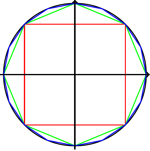
This algorithm is similar to the one we called circle, where we broke-down a disc into small squares, and counted the one which fit into a circle.

Here, we use polygons instead. They are centered and fit into a circle, and we can compute their circumference, and compare it to the diameter of the circle.

Starting with a square should be self-explanatory, and increasing the number of vertices should yield to better approximations of $\pi$.

We can translate that into C:

unsigned int i;
double polygon_edge_sq = 2.0;
unsigned long polygon_sides = 4;
for(i = 0; i < n; i++) {
    polygon_edge_sq = 2.0 - 2.0 * sqrt(1 - polygon_edge_sq / 4.0);
    polygon_sides *= 2;
}
return polygon_sides * (double) sqrt(polygon_edge_sq) / 2.0;

However, we run into an issue, where the approximation gets worse for $n \geq 14$, and fails for $n \geq 27$. Respectively equivalent to polygons with $2^15 = 65'536$ and $2^28 = 536'870'912$ vertices. We’re dealing with very numbers requiring accuracy, something floating point variables aren’t good at storing¹⁹.

Improved resolution

Let’s improve it, using the GMP library²⁰.

unsigned int i;
mpf_t polygon_edge_sq;
mpf_init(polygon_edge_sq);
mpf_t tmp;
mpf_init(tmp);
mpf_set_d(polygon_edge_sq, 2.0);

unsigned long polygon_sides = 4;
for(i = 0; i < n; i++) {
    mpf_div_ui(tmp, polygon_edge_sq, 4);
    mpf_ui_sub(tmp, 1, tmp);
    mpf_sqrt(tmp, tmp);
    mpf_mul_ui(tmp, tmp, 2);
    mpf_ui_sub(polygon_edge_sq, 2, tmp);
    polygon_sides *= 2;
}
mpf_sqrt(polygon_edge_sq, polygon_edge_sq);
mpf_mul_ui(polygon_edge_sq, polygon_edge_sq, polygon_sides/2.0);
//gmp_printf("pi: %.16Ff\n", polygon_edge_sq);
return mpf_get_d(polygon_edge_sq);

It now uses more accurate floating-point numbers with variable mantissa/exponent so the approximation only gets worse for $n \geq 50$, and fails for $n \geq 61$.

The slight downsides are that it’s more difficult to read and slower to execute.

Ramanujan

The Ramanujan-Sato²¹ series is an infinite sum of rational numbers that uses real coefficients to give $\frac{1}{\pi}$. One thing to note is that it’s from the $20^{th}$ century, shortly before computers were developped.

$$\frac{1}{\pi} = \frac{2 \cdot \sqrt{2}}{99^2} \cdot \sum_{k=0}^{\infty} \frac{(4k)!}{k!^4} \frac{26390k + 1103}{396^{4k}}$$

Since we see factorial and power operations that are likely to overflow with 64-bit variables, it’s a good idea to start directly with the GMP²² library.

That converges very fast and gives 13 digits within 3 iterations, where it reaches float’s minimum accuracy.

Chudnovsky

The Chudnovsky algorithm²³ is an update over Ramanujan’s algorithm, that’s still used for computing large numbers of $\pi$ digits using computers.

$$\frac{1}{\pi} = 12 \cdot \sum_{k=0}^{\infty} \frac{ (-1)^k (6k)! (545'140'134k + 13'591'409) }{ (3k)!(k!)^3(640'320)^{3k+3/2} }$$

This is supposed to converge fast and be accurate²⁴, except that my implementation stopped converging after reaching 7 digits over 2 iterations.

Plouffe

The Bailey–Borwein–Plouffe formula²⁵ is also a modern algorithm based on an infinite sum of rational numbers.

$$\pi = \sum_{k=0}^{\infty} \frac{1}{16^k} (\frac{4}{8k+1} - \frac{2}{8k+4} - \frac{1}{8k+5} - \frac{1}{8k+6} )$$

One interesting thing to note is that most terms are close to negative powers of two, and if not, their bits aren’t spread apart. This means that each partial sum can be accurate, even using standard precision floating-point numbers²⁶. High resolution is only needed when summing partial sums.

This reached 18 digits accuracy after 14 iterations.

Bellard

Bellard’s formula²⁷ is an improvement over the Plouffe formula that works in a similar way, using lots of terms that are based on powers of 2.

$$\pi = \frac{1}{2^6} \sum_{k=0}^{\infty} \frac{(-1)^k}{2^{10n}} ( -\frac{2^5}{4k+1} -\frac{1}{4k+3} + \frac{2^8}{10n+1} -\frac{2^6}{10n+3} -\frac{2^2}{10n+5} -\frac{2^2}{10n+7} +\frac{1}{10n+9} )$$

This is even faster than Plouffe’s formula, where it reached 20 digits accuracy after 7 iterations.

Helping functions

Some of the previous algorithms require external functions that are generic and can be reused.

Short functions can use the inline keyword²⁸, meaning that the compiler will try to replace it in the code to avoid function calls, in a way to improve performance, with depth and length limitations.

Factorial

The factorial function is needed for N-Sphere and Newton algorithms.

By definition, $n! = \prod\limits_{k=1}^{n} k = n \cdot (n-1) \cdot ... 2 \cdot 1$, and $0! = 1$.

Iterative

Let’s translate that in C with a loop:

inline unsigned long factorial_(unsigned long n) {
    unsigned long fact = 1;
    unsigned long i = 0;
    for(i = n; i > 0; i--) {
        fact *= i;
    }
    return fact;
}

Recursive

We can also write it in this way, with a recursive function that calls itself:

inline unsigned long factorial(unsigned long n) {
    if(n > 1)
        return n*factorial(n-1);
    if(n <= 1)
        return 1;
    return 0;   // never happens
}

The reason why both ways have been tried is to compare their performances, where the recursive method is supposed to use more memory space, but executes faster.

Double Factorial

Double Factorial is called Factorial2 here, to avoid confusion with variable types. It’s very similar to factorial, except that it skips evey second iteration:

By definition, $n!! = n \cdot (n-2) \cdot ... 4 \cdot 2$ for even numbers, $n!! = n \cdot (n-2) \cdot ... 3 \cdot 1$ for odd numbers, and $0!! = 1$.

No need to compare recursive and iterative methods, let’s directly write a recursive function:

inline unsigned long int factorial2(unsigned long int n) {
    if(n > 2)
        return n*factorial2(n-2);
    if(n <= 2)
        return 1;
    return 0;   // never happens
}

Binomial coefficients

We need binomial coefficients²⁹, $\binom{n k} = \frac{n!}{(n-k)!}$, and since we already have a factorial function, the code is super easy:

inline unsigned int binomialc(unsigned int n, unsigned int k) {
    return factorial(n)/(factorial(k)*factorial(n - k));
}

References

---

1. Comparaison de langages de programmation : Méthode Monte-Carlo↩︎

2. Comparaison de langages de programmation (5) : Surface d’un disque↩︎

3. n-sphere - Wikipedia↩︎

4. Volume of an n-ball - Wikipedia↩︎

5. Comparaison de langages de programmation (5) : Surface d’un disque↩︎

6. Pascal’s triangle - Wikipedia↩︎

7. Taylor series - Wikipedia↩︎

8. Machin-like formula - Wikipedia↩︎

9. The GNU Bignum Library↩︎

10. Leibniz formula for $\pi$ - Wikipedia↩︎

11. Basel problem - Wikipedia↩︎

12. Riemann zeta function - Wikipedia↩︎

13. Double-precision floating-point format - Wikipedia↩︎

14. Arithmetic–geometric mean - Wikipedia↩︎

15. Gauss–Legendre algorithm - Wikipedia↩︎

16. Gauss–Legendre algorithm - Wikipedia↩︎

17. Arbitrary-precision arithmetic - Wikipedia↩︎

18. The GNU Bignum Library↩︎

19. Double-precision floating-point format - Wikipedia↩︎

20. The GNU Bignum Library↩︎

21. Ramanujan–Sato series - Wikipedia↩︎

22. The GNU Bignum Library↩︎

23. Chudnovsky algorithm - Wikipedia↩︎

24. Pi - Chudnovsky - Nick Craig-Wood↩︎

25. Bailey–Borwein–Plouffe formula - Wikipedia↩︎

26. Double-precision floating-point format - Wikipedia↩︎

27. Bellard’s formula - Wikipedia↩︎

28. An Inline Function is As Fast As a Macro - GCC↩︎

29. Pascal’s triangle - Wikipedia↩︎

• ← Previous page
  Disjoncteur Magnéto-Thermique
• Next page →
  cms

Electronics Électronique puissance semiconducteur semiconductors power Hardware CPE INSA Xavier Bourgeois

Xavier